I love using Strava to track my bike rides, it's light on the battery, and there's even a handy little homescreen widget I can use to start up a new ride. Now on top of that, I found out that they also let you download all your activity history, which is great because I've been wanting to familiarize myself a little bit with Jupyter/Pandas/Matplotlib lately. It's actually pretty neat, and you can get some interesting results pretty quickly.

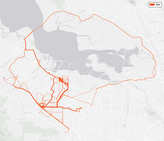
A heat map of my tracked bike rides around the Bay Area. The loop around the bay is a good ride, except for a small patch just past the Dumbarton Bridge where it is not paved.

The dump from Strava is provided as a zip of GPX files, one for each tracked activity including metadata and raw waypoint data (lat/long, elevation, time, etc). The waypoint data is suprisingly precise and abundant, I had over 560k waypoints for the only 300+ rides since I started tracking, and from that you can pretty easily calculate the basic Strava information from their site; distance of each ride (using the Haversine formula as I found out), average speed, elevation climb, and moving time for example.

In my case, I wanted more information about my commute, so I broke down the rides into the three categories; morning, evening and leisure, and by joining that with some weather data from Darksky, I found some pretty interesting things about my rides.

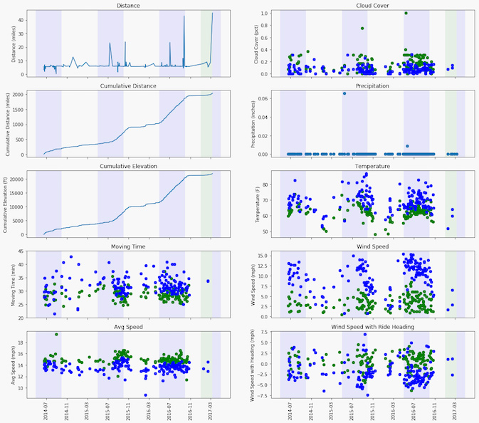
Some descriptive statistics of my riding data. The wind speed with heading was approximated by taking the dot product of the wind vector (at the ride start) and the normalized ride vector scaled by the wind speed.

Each point in the plots is a ride; green for a morning commute and blue for an evening commute. The blue backgrounds indicate "summer" months, and the green-ish background indicates the current year. From a first glance, you can see that I don't really ride in the rain (hence no precipitation data :), and the majority of my tracked rides are accounted for by commutes to and from work. If you add up the cumulative elevation change, I've also ridden higher than Mt. Fuji now, which is pretty cool!

Looking at the rest of the data, I can also find things that correlate with my experience riding over the last couple years. It's clear that I am about 2mph (2-3min) faster riding to work than from it. I've always blamed it on end-of-day tiredness and the elevation change getting back up the hills towards the Santa Cruz mountains, but it looks like there are an additional environmental effects. The increase in average temperature (10°F) doesn't help, nor does wind from the Pacific in the early evening blowing opposite to my riding direction, which I had never thought much about until now looking at the graph.

I have some more ideas for how to play with the data, but now I really wish Strava had been around back in 2007-2010 when I was riding my bike to downtown Toronto for work – that data would have been really interesting to see!

I've always wanted to play around with full-text search using Lucene or Sphinx, but never really had any reason to do so. In addition, most of those packages require having a persistent search server process to index and query from, which is extra overhead on the lean servers that I use. But since I had a bit of time these past couple days, I've been playing with around with a completely file-based full-text searching Python library called Whoosh, with my blog posts as the search corpus.

Out of the box, Whoosh has a sane setup and supports complex schemas with a variety of indexable, stored, and weighted fields. Adding documents to the search index is fast, and querying is straightforward across multiple fields. The library also has a few interesting plugins to do things like stemming (to allow searching variants of a base word), and query correction (to propose correct spellings from either a dictionary or the content in a particular field). Whoosh is one of those Python modules that Just Works™, and it is awesome.

To see it in action, try searching using the input box below. It should show snippets from each article that matches the terms, and also suggest corrected queries if there are no results found (ie. try doing a search for a typo of California).

Under the hood, Whoosh supports a variety of scoring functions including BM25F and base TF-IDF. TF-IDF is actually a pretty simple and intuitive function, one part representing the number of documents that a search query term appears in (document frequency), and the other being the frequency of the term in each document (term frequency). The more unique a term is across documents, the more likely its documents should score higher (hence, the inverse document frequency), and likewise, the more times the term is referenced in a document, the higher the score.

BM25 builds off TD-IDF, but the term frequency is effectively weighted less for high frequencies (it approaches a limit faster), and the inverse document frequency also takes the length of each document into account relative to the average document length (as longer documents will generally have more terms). As a result, the same number of terms appearing in a shorter document will score higher than in a long document. BM25F is an improvement over BM25 and supports scoring of terms across multiple weighted fields (ie. title, body, etc). Despite being from the 80's, BM25 seems to perform quite well!

One funny issue that I ran into during testing was that I could search for every month by name except for the month of "May". Stumped, I thought there was something wrong with Whoosh, until I read the docs a little closer. When using the StemmingAnalyzer, the default set of stop words (common words filtered out due to their prevalence) included "may" in the list. Removing it from that list did the trick, and all the months were fair game again. :)

Mt. Hamilton, near San Jose

McWay Falls, Julia Pfeiffer Burns State Park (near Big Sur)

One of my favourite shots, taken on Highway 190, between Bakersfield and Death Valley National Park. The area is dead quiet except for the wind, and the road runs into the distance each way you look.

Along the iconic Highway 1

A view from the Lick Observatory

California is so pretty. From the Mojave desert to the Sierra mountains to the Pacific coast, there is so much variety of landscapes in the state. For me, it'll never quite replace the majestic Rockies of southern Alberta where I grew up, but California really is a special place (at least geographically) to live.

Now if only the rents weren't so darn high!